namandangi.github.io

Diabetes Risk Prediction

Team 23

Naman Dangi, Netra Ghaisas, Hubert Pan, Hajin Kim, Pooja Pache

Video Presentation

Presentation link

Introduction:

Diabetes is a serious chronic disease that can lead to reduced quality of life and life expectancy. Type 2 diabetes typically develops in adulthood and can often be managed with lifestyle changes and/or medication. Prediabetes is a condition which entails higher blood sugar levels than normal but not high enough to be classified as type 2 diabetes. The CDC has indicated that as of 2019, 37.3 million Americans have diabetes and 96 million have prediabetes, and 1 in 5 diabetics and 8 in 10 prediabetics are unaware of their risk [2].

Complications like cardiovascular disease, vision loss, lower-limb amputation, and kidney disease are associated with chronically high blood sugar levels for those with diabetes [3]. Predictive models can assist medical professionals in identifying patients who pose a high risk of developing diabetes even before symptoms show up, enabling early intervention and treatment to prevent or delay the onset of associated complications.

We plan on using the Diabetes Health Indicators dataset from Kaggle [1] and will be predicting the Diabetes_012 column based on the other columns. The dataset is based on 253,680 survey responses from the CDC’s BRFSS2015 survey.

Problem Definition:

Identifying individuals who have or at high risk for diabetes is a critical component for public health initiatives that deal with diabetes.

For this project we plan on using the Diabetes Health Indicators dataset to:

• Build models that accurately predict if someone has diabetes or pre-diabetes
• Identify if there are any features that are more highly correlated with diabetes than others

Methods:

Initially, data cleaning and preprocessing will be our fundamental tasks. After data transformation of raw data into a usable format, we will split the dataset into a train (80%) and test (20%) set using Python libraries. As part of this process we may sample the data in a way to remedy the class imbalance that is present in the data. Further, we aim to implement five algorithms for: Supervised and Unsupervised learning. We decided to use Logistic Regression, Decision Trees and Random Forest algorithms for supervised learning while, for unsupervised learning, we intend to use K Means clustering and Gaussian Mixture Model. Additionally, we plan on data visualization, feature exploration, and comparing accuracy scores of the different supervised and unsupervised algorithms we have used for diabetes prediction.

Data Pre-Processing and EDA

To start with, we used Python’s Pandas and NumPy libraries to load and explore the dataset. For visualizations, we used Matplotlib and Seaborn libraries. As part of pre-processing, we checked for data types, missing and null values, duplicate values and class imbalances. To find correlation between features and diabetes risk, we drew up a correlation matrix and various plots, which we elaborate on in the Results and Discussion section

Supervised:

A. Logistic Regression

In our initial data analysis, we applied the logistic regression algorithm to our large dataset and opted for the SAGA (Stochastic Average Gradient Descent) solver instead of the default LBFGS (Limited-memory Broyden-Fletcher-Goldfarb-Shanno) solver. This decision was based on SAGA’s support for L1 regularization, which can help with feature selection and reducing overfitting. However, we encountered overfitting and to address it, we employed both SMOTE oversampling and Stratified K-fold undersampling techniques. To further enhance our model’s accuracy, we utilized PCA for dimensionality reduction. We experimented with different combinations of the number of PCA components and the number of folds, monitoring their impact on recall, accuracy, roc score and explained variance.

B. Random Forest

Initially, we split our data into an 80:20 ratio for the train-test set and started the implementation of our random forest model using the basic RandomForest Classifier without any hyperparameters. We then fine-tuned the hyperparameters using the RandomForestClassifier and used RandomizedSearchCV to find the best parameters and best estimators. Additionally, we also tried the BalancedRandomForestClassifier approach to enhance the model’s accuracy. Furthermore, we implemented various techniques such as SMOTE, SMOTEENN, Undersampling, and Stratified K-fold to augment the accuracy of our model.

C. Decision Trees

For decision trees we went with a 20/80 test split stratified by the Diabetes_012 label. We also used SMOTE to generate an alternative test and train set to take into account the severe imbalance between the different data set classes (but ultimately did not use it). We then repeatedly created entropy reduction based decision trees with maximum heights ranging from 1 to 32 to determine which maximum height yielded the best accuracy.

Unsupervised:

A. KMeans

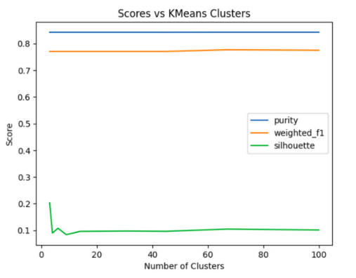
As part of the initial data exploration we also ran the KMeans algorithm on the dataset to explore how well the data was partitioned. This was done via the “elbow method” by repeatedly running KMeans multiple times with different numbers of clusters, evaluating those clusters against a set of metrics, and then looking at how increasing the target cluster count affected the measured cluster evaluation scores by graphing the results. For the purposes of this study we looked at the following cluster evaluation scores: purity, weighted f1, and silhouette across the geometric sequence from 3 to 100. Initially, data cleaning and preprocessing will be our fundamental tasks. After data transformation of raw data into a usable format, we will split the dataset into a train (80%) and test (20%) set using Python libraries. As part of this process we may sample the data in a way to remedy the class imbalance that is present in the data. Further, we aim to implement five algorithms for: Supervised and Unsupervised learning. We decided to use Logistic Regression, Decision Trees and Random Forest algorithms for supervised learning while, for unsupervised learning, we intend to use K Means clustering and Gaussian Mixture Model. Additionally, we plan on data visualization, feature exploration, and comparing accuracy scores of the different supervised and unsupervised algorithms we have used for diabetes prediction.

B. Gaussian Mixture Model

For GMM we first used PCA to reduce the number of features from twenty two to three and then used the sklearn GaussianMixture implementation to fit a Gaussian Mixture Model to the resulting data. Lastly, the silhouette score and Davies-Bouldin index were used for evaluating the accuracy.

Potential Results and Discussion:

For the project, we plan to conduct a comparative analysis of the performance of the various models. In order to accomplish this, we will take into consideration a range of potential factors, such as Confusion Matrix, Accuracy, ROC Curves, mutual information scores, and mean squared error. The specific metrics used for this comparison will be determined by the models chosen for evaluation. In terms of results, it is anticipated that certain machine learning algorithms will demonstrate superior performance in relation to others. We might need to address class imbalance, duplicates, missing values, data normalization, and determining optimum number of clusters based on further analysis of the dataset.For the project, we plan to conduct a comparative analysis of the performance of the various models. In order to accomplish this, we will take into consideration a range of potential factors, such as Confusion Matrix, Accuracy, ROC Curves, mutual information scores, and mean squared error.

Data Pre-processing

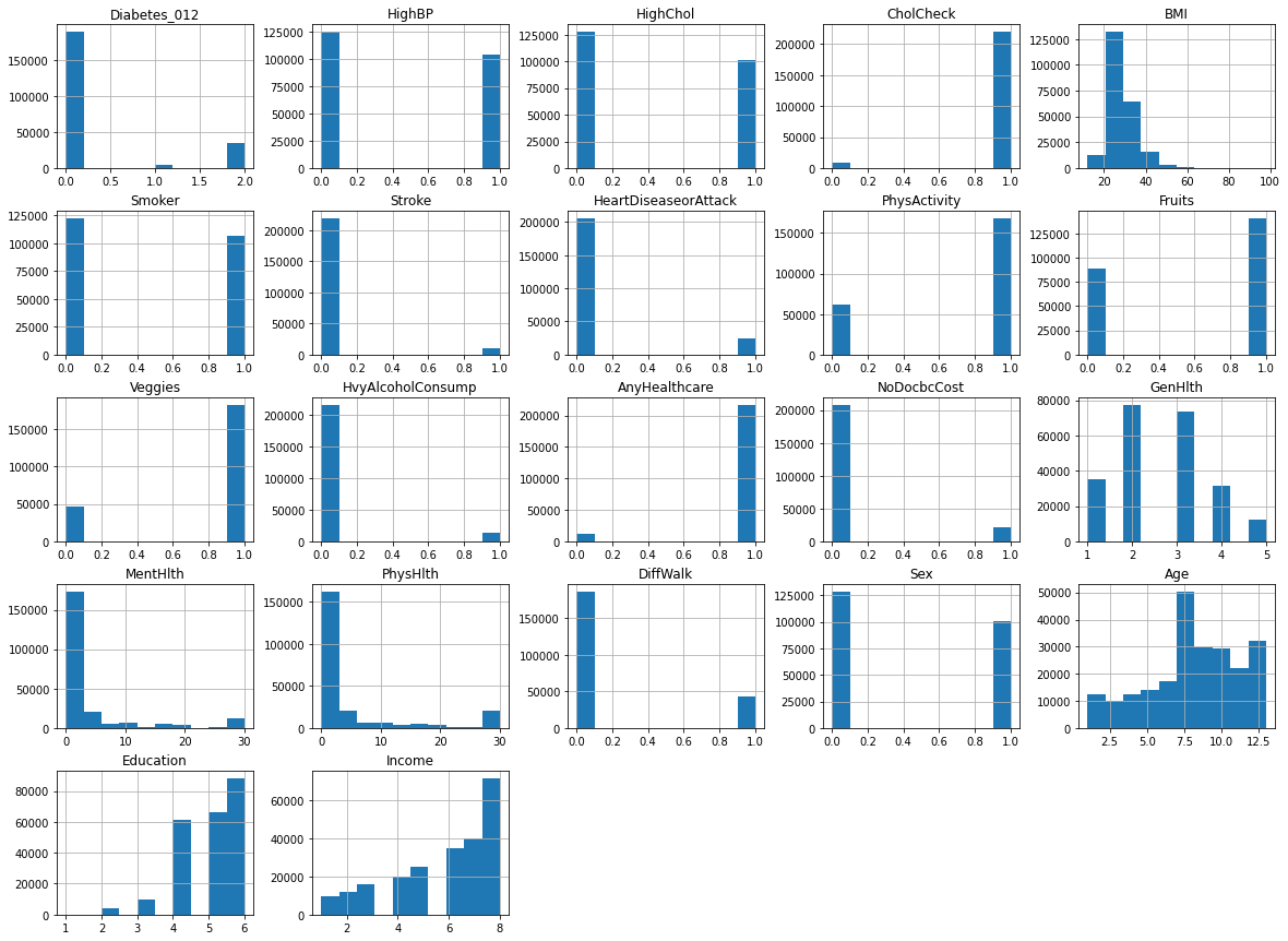
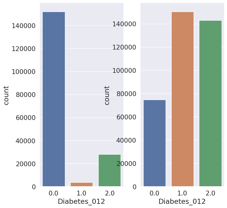
Based on the given information, we can infer that the dataset contains a total of 22 features, including 22 discrete and 7 continuous variables, and the target variable is Diabetes_012. The dataset is represented using a histogram, which shows the distribution of the variables.

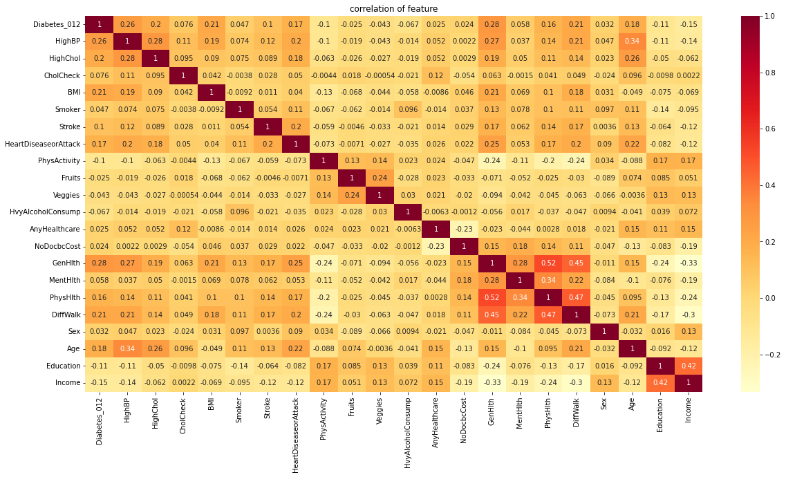
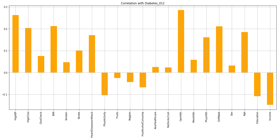
To identify the most influential features for diabetes, a feature correlation heatmap and bar plot were used. The heatmap and bar plot suggest that HighBP, HighChol, BMI, Stroke, GenHlth, MentHlth, PhysHlth, Age, Education, and Income are the most influential features for diabetes. This means that these variables have a strong correlation with diabetes, and may be used to predict the likelihood of someone developing diabetes.

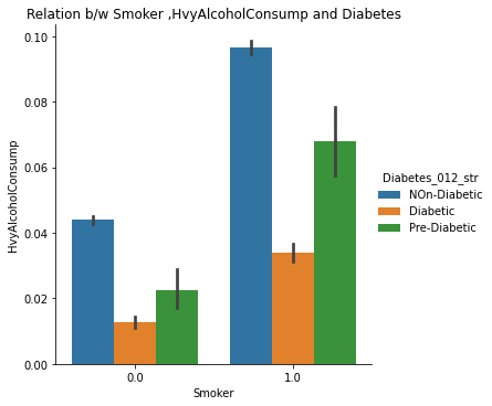
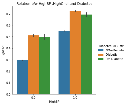
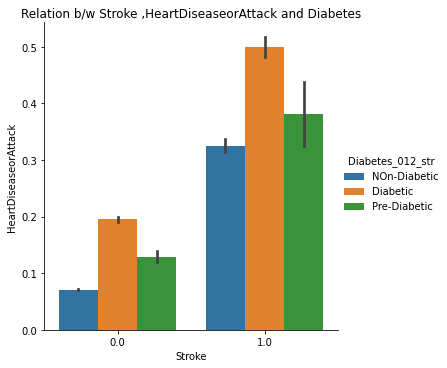
The catplots for Smoking and HvyAlcoholConsump, Stroke and HeartDiseaseorAttack, and HighBP and HighChol suggest that these variables, when present together, increase the risk of diabetes. This indicates that individuals who have these variables are more likely to develop diabetes than those who do not.

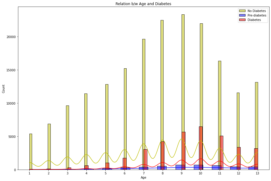
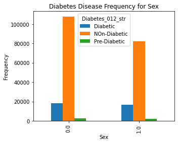
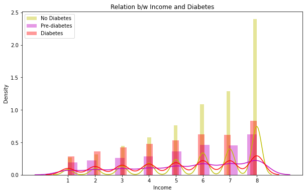
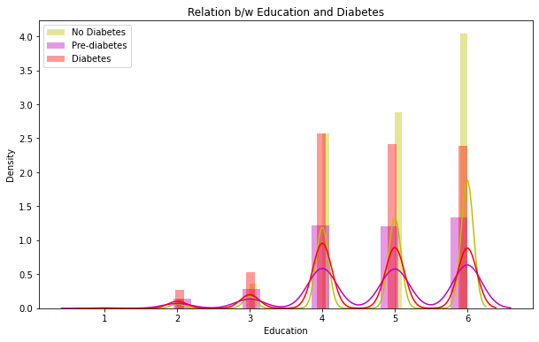
The distplots and boxplots suggest that the risk of diabetes is equally high for both males and females. However, people who are aged 45 and above are more susceptible to diabetes and pre-diabetes. Additionally, individuals with lower education and income are also at a higher risk of developing diabetes.

Overall, this information suggests that diabetes is a complex disease that can be influenced by a variety of factors. The most influential features for diabetes include HighBP, HighChol, BMI, Stroke, GenHlth, MentHlth, PhysHlth, Age, Education, and Income. Individuals who have these variables, especially those who have multiple variables together, are more likely to develop diabetes. Additionally, age, education, and income are also important factors to consider when predicting the risk of developing diabetes.

1. Features

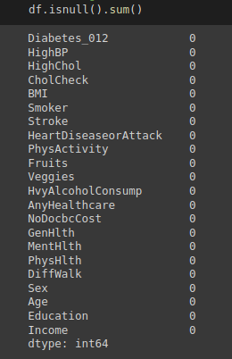
2. No Missing Values

3. Influential

4. Relation between Age and Diabetes

5. Relation between Gender and Diabetes

6. Relation between Income and Diabetes

7. Relation between Education and Diabetes

8. Checking Combined Effects of Smoking and Heavy Alcohol Consumption

9. Checking Combined Effects of High Blood Pressure and High cholesterol

10. Checking Combined Effects of Stroke and Heart Disease Attacks

During the data preprocessing stage, we did not detect any null values, but we did come across duplicate rows.

Supervised Learning

A. Logistic Regression

After evaluating the performance of the Logistic regression algorithm on our dataset, we discovered a class imbalance issue where the recall value for the Pre Diabetes class was zero.

Accuracy: 0.827817307483082

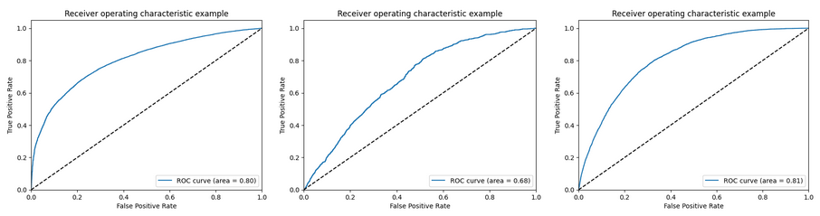
ROC curves for non-diabetes, pre-diabetes and diabetes classes

To address this issue, we applied the SMOTE oversampling and Stratified K-fold undersampling techniques separately, but both techniques individually resulted in higher accuracies but lower recall and precision metrics for the Pre Diabetes class.

Classification report after applying SMOTE

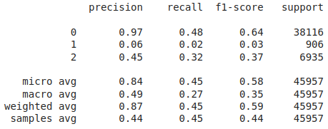
Accuracy: 0.44358857192593076

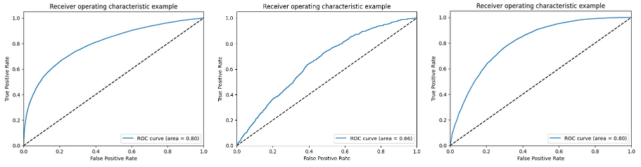
ROC curves for logistic regression after applying SMOTE oversampling technique to handle class imbalance

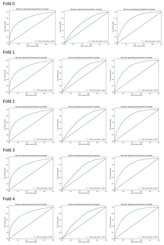
ROC curves for logistic regression after applying Stratified K-Fold cross-validation technique to handle class imbalance

For K = 5, mean accuracy: 0.8252553489240425

A combination of both techniques demonstrated better results, although the accuracies were not optimal.

ROC curves for logistic regression after applying SMOTE and Stratified K-Fold cross-validation techniques to handle class imbalance

For K = 5, Mean Accuracy: 0.44293480446825706

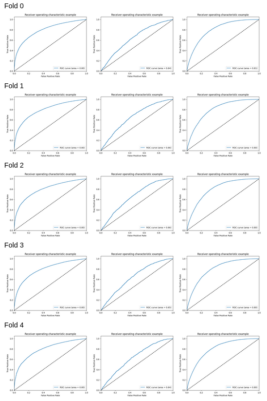
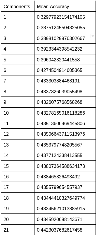
Additionally, we observed that varying the number of PCA components affected the accuracy and ROC score, with the Non-diabetic and diabetic classes achieving the highest scores when the number of PCA components equaled the total number of features.

The explained variance also increased as the number of PCA components increased.

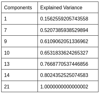
However, utilizing all components can be computationally expensive and may not produce an optimal model.

In addition, modifying the number of folds in the Stratified K-fold undersampling technique had a minor effect on accuracy. However, increasing the number of folds can lead to increased computational complexity, prolonged processing times, and greater sensitivity to noise in the data. Consequently, based on the performance metrics of Logistic regression, we concluded that it is not the most effective supervised learning algorithm for our diabetes dataset, and we intend to investigate other algorithms for improved performance.

B. Random Forests:

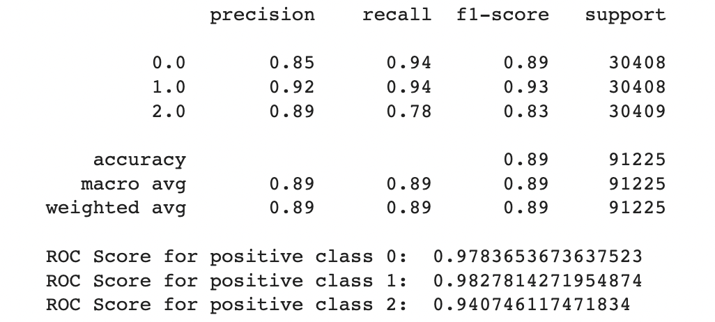
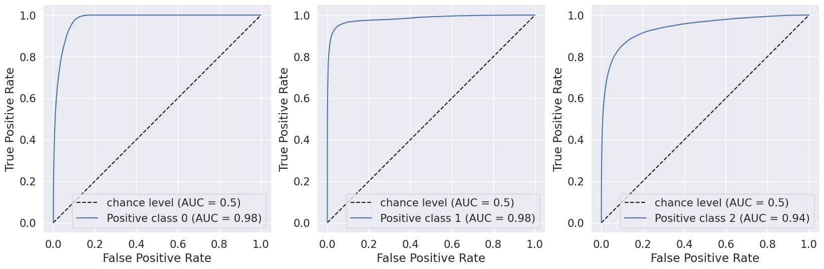
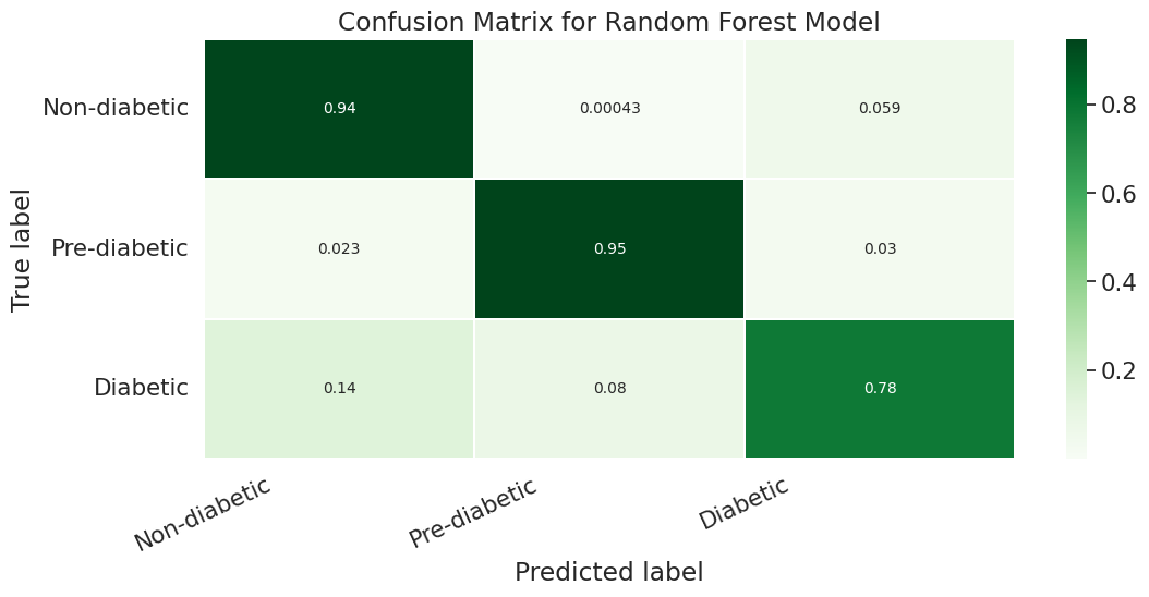
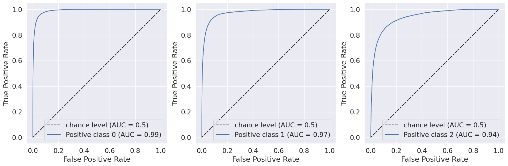
We evaluated the performance of our random forest model using classification report, confusion matrix, and AUC-ROC scores. Initially, we implemented the model without any hyperparameters and achieved an accuracy of 82.4%. However, the recall value for the Pre-diabetes class (label = 1) was 0.0, indicating a class imbalance issue in our dataset.

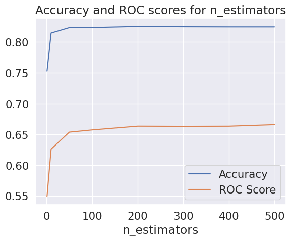
To improve the accuracy, we tuned the hyperparameters, including the n_estimators of our Random Forest classifier. We found that the accuracy started to flatten at n_estimators = 100, and the ROC scores flattened at n_estimators = 300.

We then used RandomizedSearchCV to test different hyperparameters and select the best ones. This approach yielded an accuracy of 83.6% and a ROC AUC score of 76.82%, using the best estimator with hyperparameters {‘n_estimators’: 500, ‘min_samples_split’: 6, ‘min_samples_leaf’: 10, ‘max_depth’: 60}.

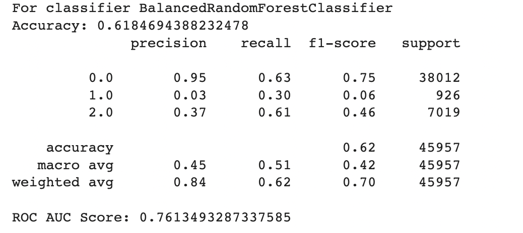
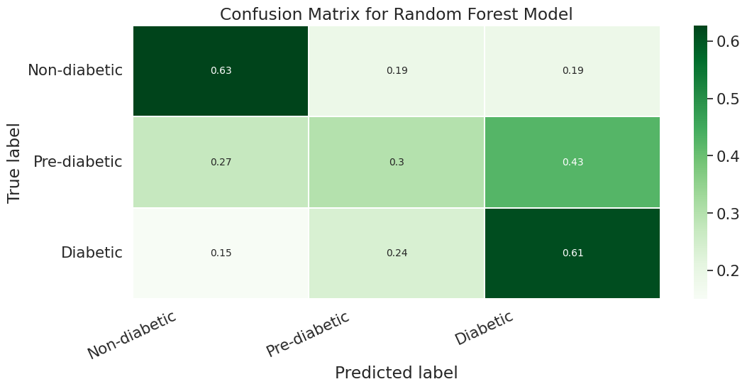
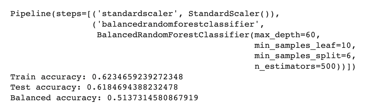
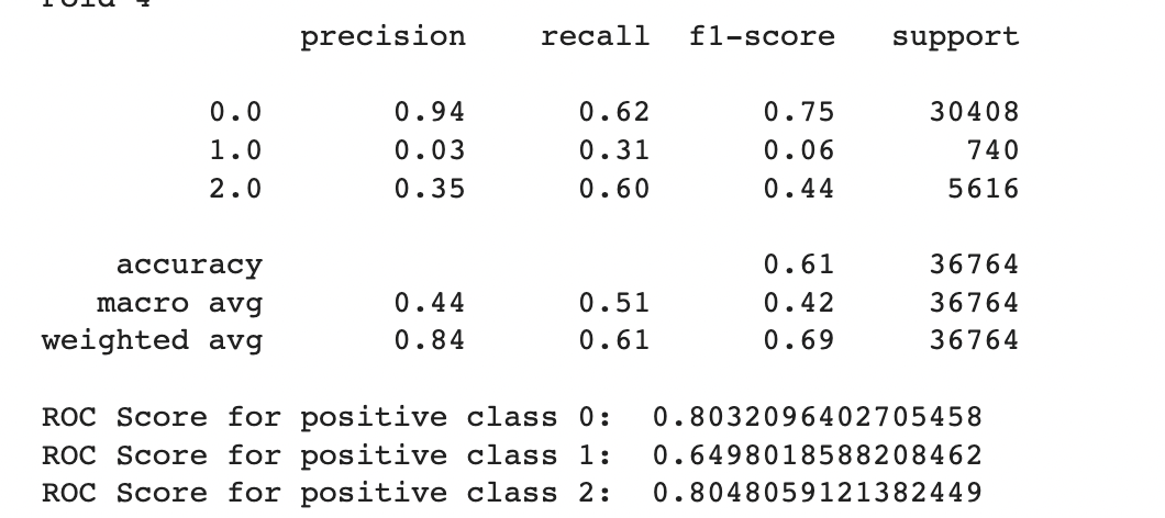
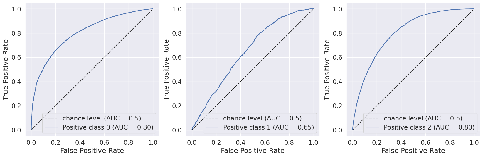
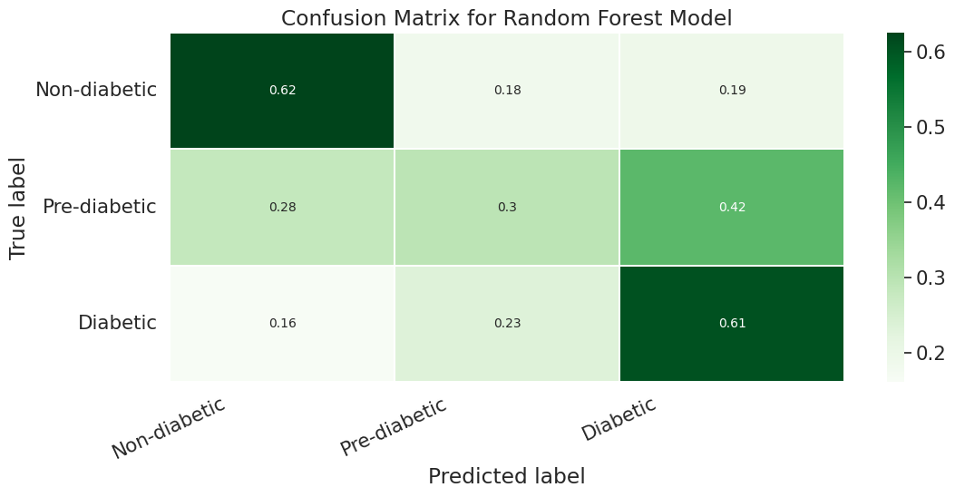
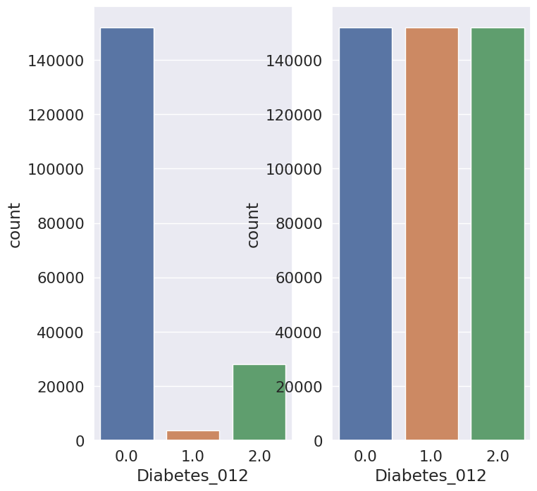
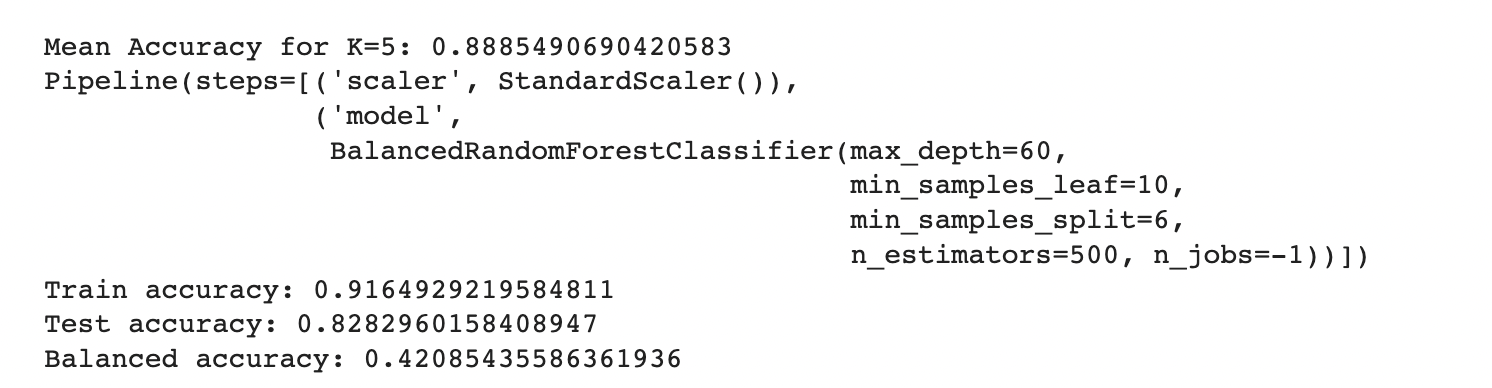
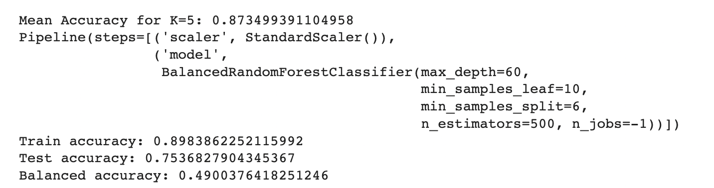
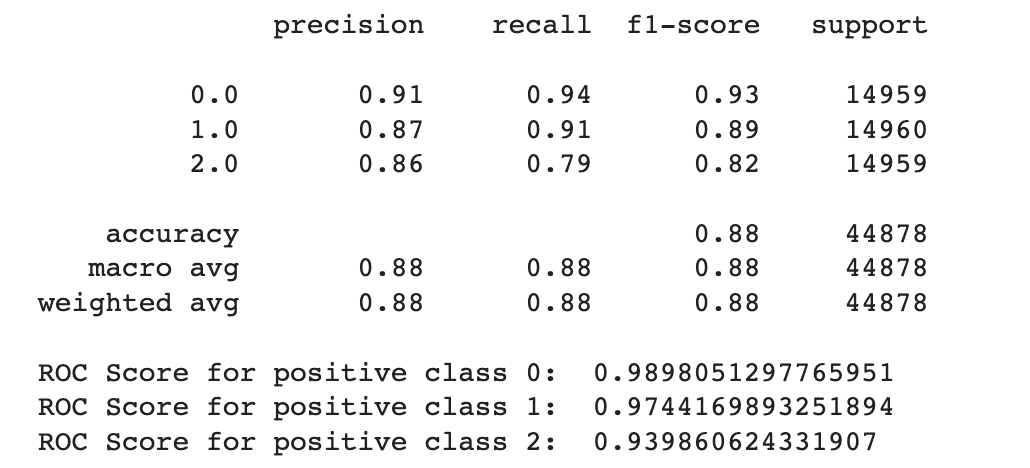
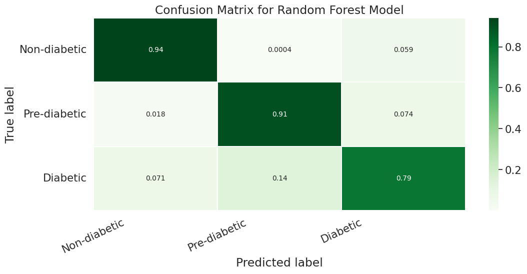
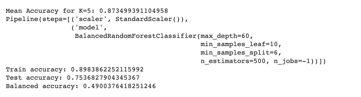
To further enhance the model performance, we tried several techniques, such as BalancedRandomForestClassifier, which randomly undersamples each bootstrap sample to balance it. However, this approach gave a low overall accuracy of 62% as compared to the baseline model’s 83%. It did show significant improvement in recall for pre-diabetes and diabetes classes and better-balanced accuracy (51%) than the baseline (37%). Following are the results we obtained for BalancedRandomForestClassifier:

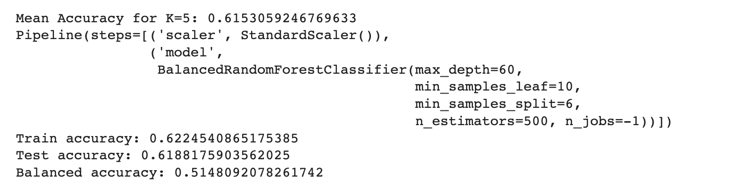
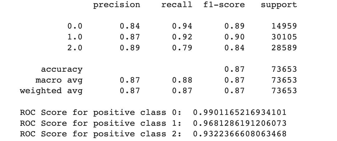
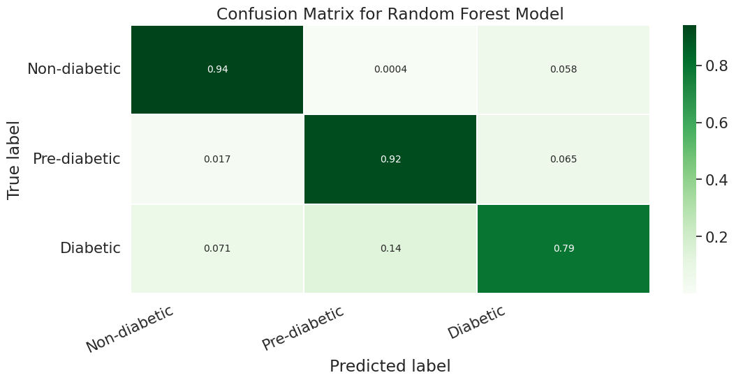
We also used Stratified Kfold validation with the number of K-folds = 5, a combination of SMOTE and stratified K-fold, a combination of SMOTEENN and Stratified K-Fold pipeline, and a combination of SMOTE, Random undersampling, and Stratified K-Fold pipeline. We observed that the Stratified K-fold slightly improved the balanced accuracy compared to the BalancedRandomForestClassifier. Following are the results we obtained for Stratified K-fold:

However, SMOTE and SMOTENN caused the model to overfit, with a balanced accuracy (42%) much lower than the training accuracy (91.6%). The last approach, where we applied Undersampling after applying SMOTE and SMOTEENN, reduced overfitting, but the balanced accuracy decreased.

A.Results for combination of SMOTE and Stratified K-fold:

B.Results for combination of SMOTENN and Stratified K-fold:

C.Results for combination of SMOTENN, Random undersampling and Stratified K-fold:

C.Decision Trees

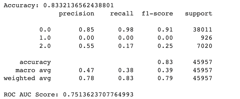
As seen in the relevant Python notebook, the max depth with the highest accuracy of 0.8332136562438801 was 8. This indicates that extending the depth of the decision tree beyond 8 layers led to overfitting on the training set which resulted in poorer performance on the testing set.

Decision Tree Illustration

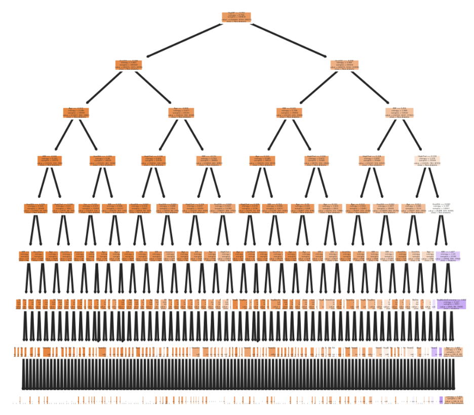
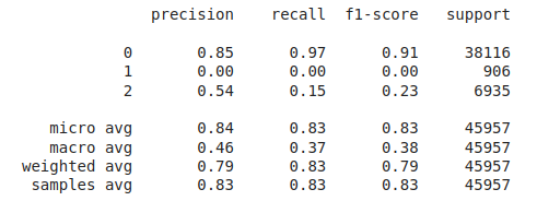
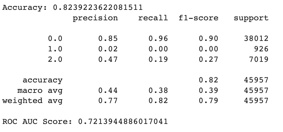
We then looked at the performance of the max depth 8 decision tree across the multiple folds and output the relevant statistics.

In general the output values for across the different folds were pretty similar with a high overall accuracy of around 0.833. As seen in the excerpted table below, the precision, recall, and f1 scores have been split out by the different label classes 0, 1, and 2. It looks like the precision, recall, and f1-score values were relatively high for the non-diabetic “0.0” class, non-existent for the pre-diabetic “1.0” class and pretty bad for the diabetic “2.0” class. This indicates that the tree model does a better job of identifying non-diabetic people versus the other classes

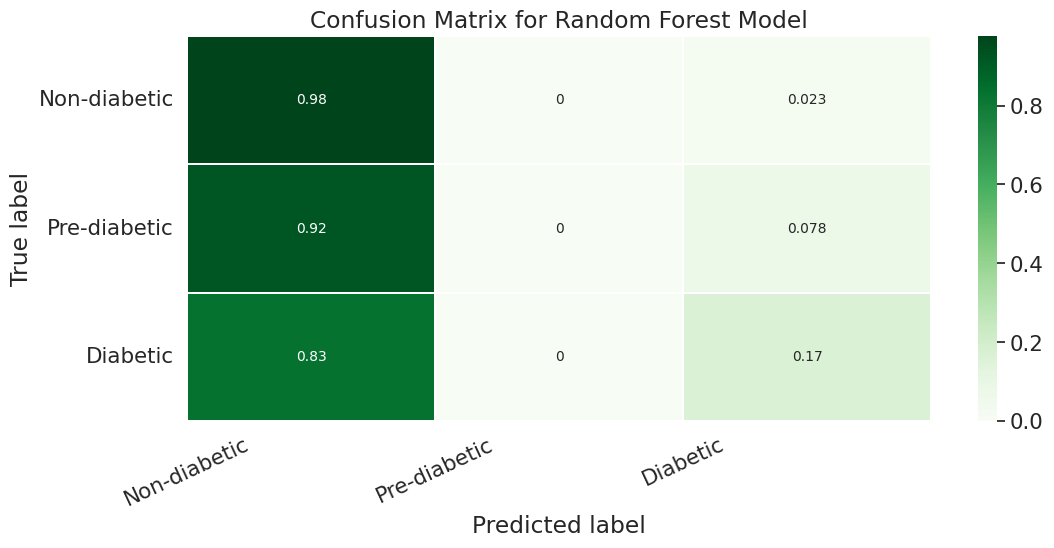
However if we look more deeply into the confusion matrix we can see that the problem is that most of the Pre-Diabetic (1) and Diabetic (2) entries are just being erroneously labeled as Non-diabetic (0). This is likely due to the fact that we did not properly even out the representation between the different partitions with smote for this particular experiment.

Unsupervised Learning

A.KMeans

The metric used to evaluate the clustering results did not show a significant improvement as the number of clusters increases. In addition, the confusion matrix reveals that all predicted clusters contain mostly points belonging to the Diabetes_012 class, indicating that the clustering algorithm is not able to identify meaningful patterns or clusters in the data. This observation suggests that a different clustering algorithm or preprocessing technique may be more suitable for this dataset. For instance, increasing the number of initializations for the K Means algorithm with larger values of K may improve the clustering results. By using larger initializations, the algorithm will generate more candidate solutions with different starting points and increase the chance of finding a good local optimum. The expectation is that the algorithm can detect more compact clusters that accurately reflect the actual partitions in the data, resulting in an enhancement of the clustering quality measurement. However, it is important to note that increasing the number of initializations and K can also lead to a longer computational time and higher memory usage.

B. Gaussian Mixture Model (GMM)

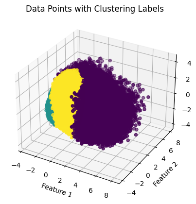
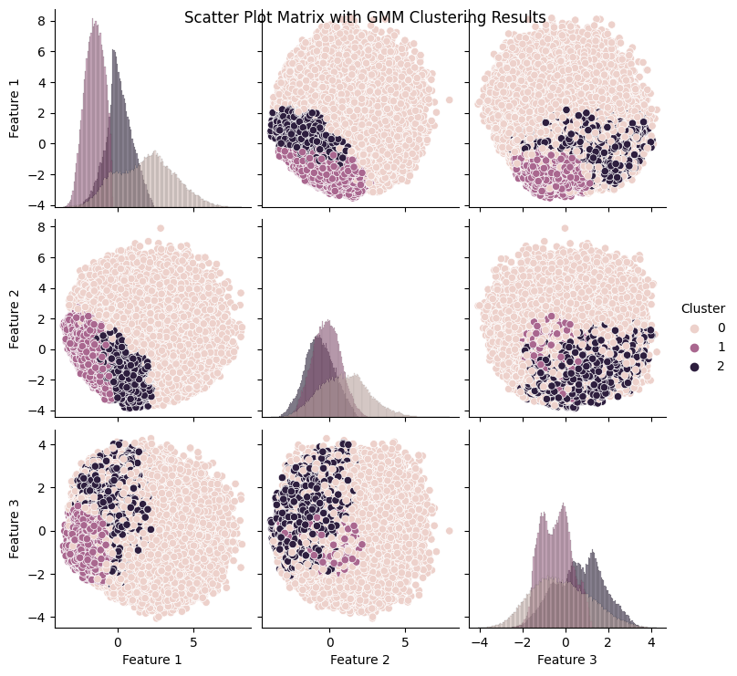
As seen in the produced graphs, using PCA to reduce the components from 22 to 3 appeared to illustrate the fact that while the different classes did tend to cluster with their similarly labeled data points. This is highlighted in the 3-D graph where the bulk of the visible yellow diabetic data points are clustered in the bottom left corner of the data point cloud. The silhouette score of 0.205 indicates that data points within the same cluster are similar, but they may also be similar to data points in other clusters. Moreover, the Davies-Bouldin index value of 1.553 indicates that the algorithm’s clusters are somewhat dissimilar to one another but not optimally distinct. The results suggest that a different clustering algorithm or preprocessing technique would be better suited to this dataset.

In addition, as evidenced in the component wise plots we can see that there was a good deal of overlap between the three partitions when it came to each of the individual PCA components.

Conclusion:

Through our implementation and analysis of supervised and unsupervised algorithms, we gained several valuable insights. Firstly, we found that highly imbalanced classes can result in models generating inaccurate accuracy scores. Additionally, unsupervised techniques can be highly effective in visualizing data from a specific perspective, particularly when combined with dimensionality reduction techniques such as PCA. To prevent inaccurate accuracy scores from highly imbalanced datasets, it is necessary to adjust data using techniques like SMOTE. Moreover, supervised models typically achieved an accuracy score of around 83%. Although Decision Trees and Random Forest had similar performances, both outperformed Logistic Regression. We also found that non-supervised methods tended to produce low silhouette scores, usually below 0.2. Lastly, the slightly higher score of GMM suggests that it performed slightly better at modeling the data.

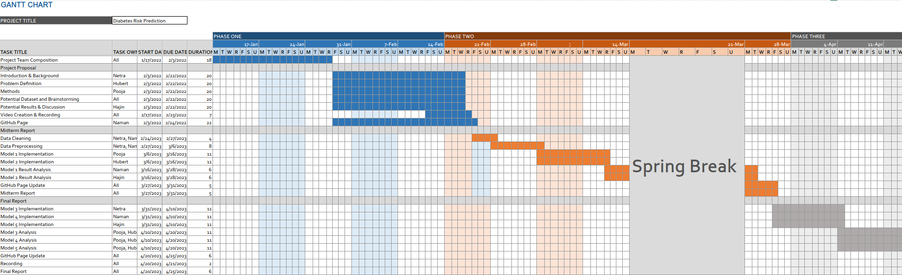
Timeline:

(Static Image Alternate)

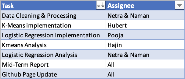
Mid-Term Contribution Table:

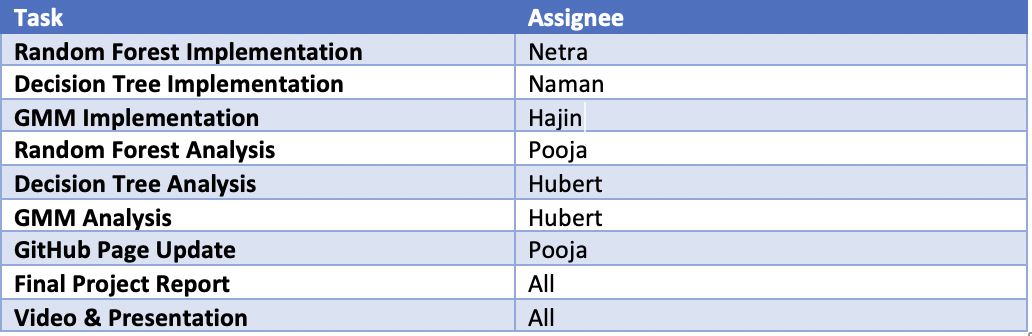
Final Contribution Table:

References:

1. Teboul, Alex. Diabetes Health Indicators Dataset. https://www.kaggle.com/datasets/alexteboul/diabetes-health-indicators-dataset. Accessed 23 Feb. 2023.
2. CDC - BRFSS - Survey Data & Documentation. 29 Aug. 2022, https://www.cdc.gov/brfss/data_documentation/index.htm.
3. American Diabetes Association; Economic Costs of Diabetes in the U.S. in 2007. Diabetes Care 1 March 2008; 31 (3): 596–615. https://doi.org/10.2337/dc08-9017
4. Xie Z, Nikolayeva O, Luo J, Li D. Building Risk Prediction Models for Type 2 Diabetes Using Machine Learning Techniques. Prev Chronic Dis 2019;16:190109. DOI: http://dx.doi.org/10.5888/pcd16.190109